
Regression: Assessing Errors
I recently saw several related errors come up in multiple presentations. The presenters claimed that:
- Deviations from normality made linear regression inappropriate to use, and
- A density estimate of your data could be useful in choosing the distributional form of your response variable (a normal distribution in this case).
Both are incorrect, but it’s worth reviewing the basics again to understand why.
Regression can be understood as a way to directly model some output \(Y\) given some information \(X\). It is natural to condition on \(X\) when doing so, since for some function \(f(x)\) of the observed \(X=x\), we have
\[\mathbb{E}[L(f(x), Y)]=\mathbb{E}\,\big[\mathbb{E} \,L(f(x)|Y)\,|\,x\big],\] and the quantity on the right gives the optimal predictor of \(Y\) as \(g(x)=\underset{a}{\text{argmin}} \big[\mathbb{E} \,L(a|Y)\,|\,x\big].\)
That is, \(g(x)\) is the intended “regression function” we wish to achieve and it is conditional on a realized unit of information \(x\). This leads us to treat error distributions as fixed, given a particular \(x\) value.
First Practical Example
Say you run across the following data, plotted with a density estimate:
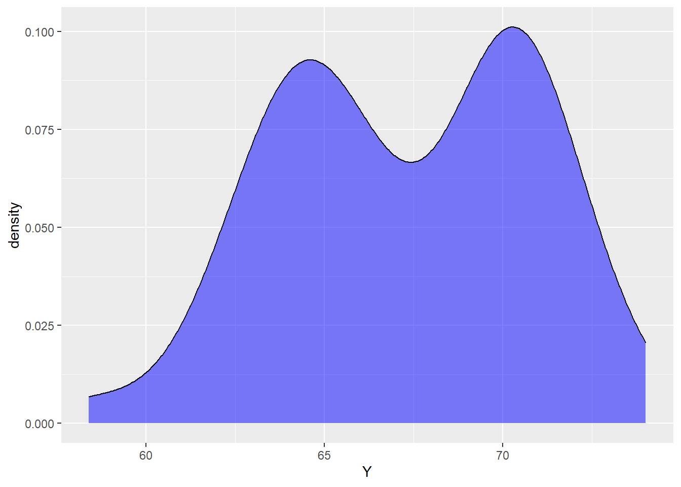
The data are clearly not normal right? If you were to run a K-S test or make a qqplot for the data, you may reject the assumption of normality.
However, given some information \(x\), the data could look normal:
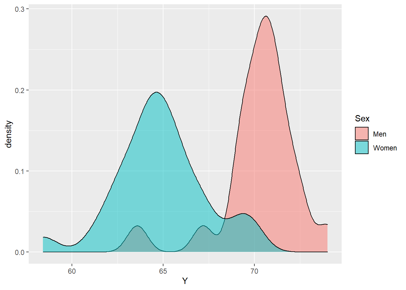
The point I am making here is a simple one: a marginal pictures of your data may not be useful in making distributional assumptions. In fact, the data here was actually had the following mean function:
\[\mathbb{E}\,[Y_i\,|\,x_i] = \mathbb{I}[x_i = \text{Male}] \cdot 70 + \mathbb{I}[x_i = \text{Female}] \cdot 65\] If we choose to integrate out over \(x\), we obtain
\[\mathbb{E} \, \big[ \mathbb{E}\,Y_i\,|\,x_i \big] = \mathbb{E}[Y_i]= \mathbb{P}(x_i = \text{Male}) \cdot 70 + \mathbb{P}(x_i = \text{Female}) \cdot 65.\]
This is a mixture of mean functions depending on the probabilities of \(X\). Moreover, if the data are normal given \(X=x\), the data are not normal marginally.
Zero-inflated Poisson
Count data are said to follow a zero-inflated poisson distribution if they are a mixture of a poisson distribution and Dirac measure at 0. If one is to use a Poisson random component, the typical advice is to check if there are “too many” zero values to be accommodated.
When the models become more complex, however, checking for zero-inflation becomes more difficult (and again, a marginal picture won’t help!). Consider, for instance,
\[Y_i|\pmb{x}_i \sim \text{Poisson}(\eta_i)\]
\[\log[\eta_i] = \pmb{x}_i^T \beta\]
Here, the Poisson assumption depends on the appropriateness of 1) the linear model in \(\beta\), 2) the link function \(\log\), and 3) the actual random component.
One may still perform checks for zero-inflation simply by simulating from a fitted model. That is, taking \(Y^{\text{rep}} \sim Poisson(\, \hat{\eta_i}\,)\) and checking the proportion of zeros from the model to the actual proportion.